Why Excel Mistakes Are Costing You More Than You Think
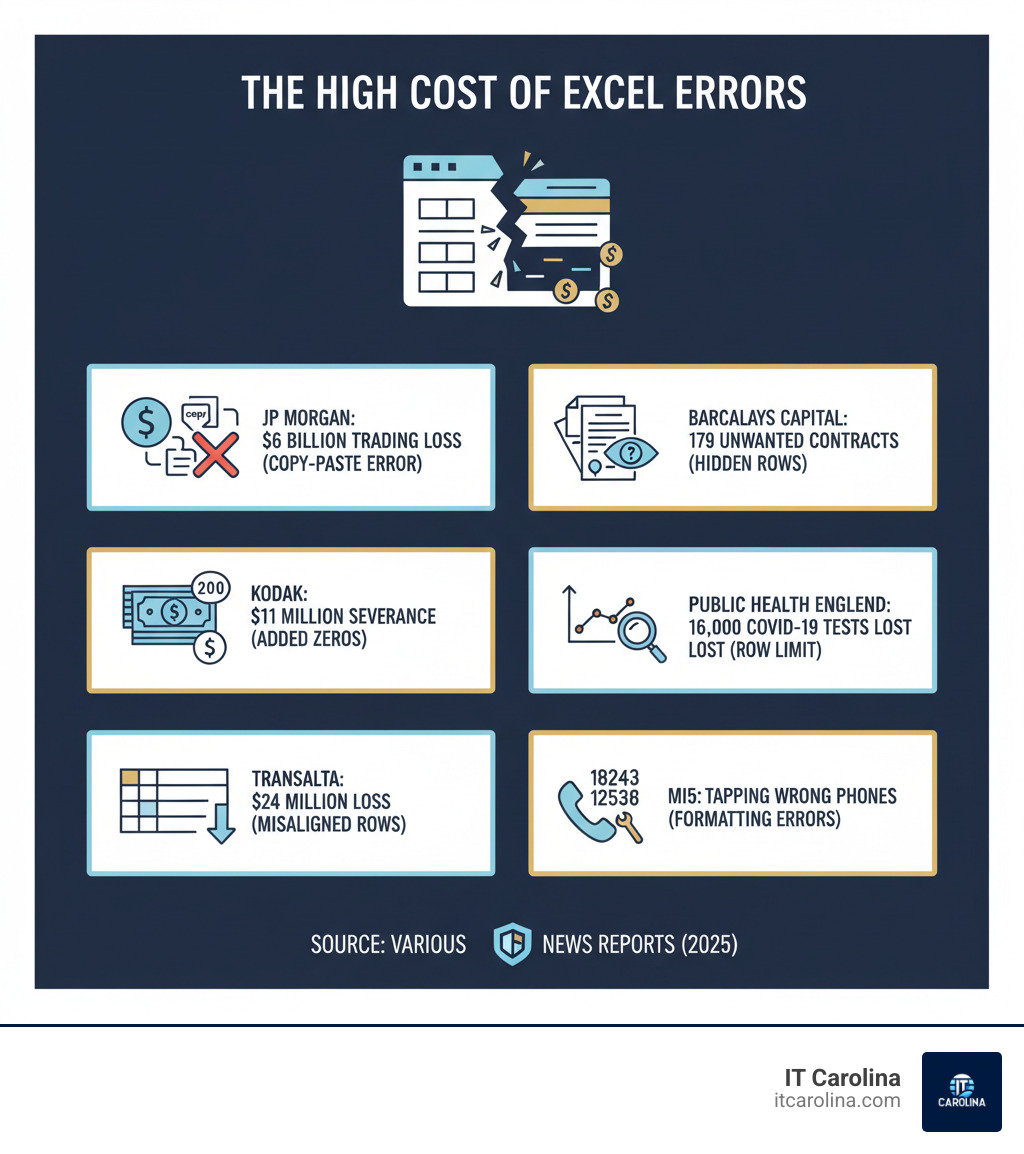
Top 10 mistakes you always do in excel spreadsheets can lead to serious financial losses, data integrity issues, and wasted time. These aren’t just minor annoyances; they’ve caused real-world damage. JP Morgan lost $6 billion from a copy-paste error, and Public Health England misplaced nearly 16,000 COVID-19 tests by hitting Excel’s row limit.
Here’s what you need to avoid:
- Merging cells – Breaks sorting, filtering, and data selection
- Using blank rows/columns – Disrupts formulas and AutoFill
- Non-tabular layout – Makes PivotTables and charts impossible
- Dates/numbers as text – Causes calculation errors
- Hardcoding values in formulas – Creates inflexible, error-prone logic
- Forgetting absolute references ($) – Produces wrong results when copying
- Not using Excel Tables – Misses automatic formatting and dynamic ranges
- Ignoring hidden data – Creates security risks when sharing
- Manually summarizing data – Loses valuable detail for analysis
- Skipping formula audits – Allows errors to go undetected
The good news is that most Excel mistakes follow predictable patterns. Once you know what to watch for, you can avoid them. This guide walks through the most common errors and provides practical, jargon-free solutions to make your spreadsheets work for you, not against you.

Foundational Flaws: How Poor Formatting and Layout Cause Errors
Spreadsheet problems often start with how the file is set up. These foundational top 10 mistakes you always do in excel spreadsheets relate to formatting and layout, making it nearly impossible to sort, filter, and analyze your data properly.
Mistake #1: Merging Cells for Titles and Formatting
Merging cells to center a title might look good, but it breaks almost everything else. Excel’s sorting, filtering, and copy-paste functions rely on a consistent grid structure. Merged cells create a block that disrupts this grid, causing sorting to fail, filters to become unreliable, and copy-pasting to become a minefield.
The solution is “Center Across Selection.” This gives you the same visual result without breaking your spreadsheet. Select the cells you want your title to span (e.g., A1 to D1), press Ctrl+1 to open “Format Cells,” go to the “Alignment” tab, and choose “Center Across Selection” from the “Horizontal” dropdown. Your title is now centered, but the cells remain separate and functional.

Mistake #2: Using Blank Rows and Columns for Spacing
Adding blank rows or columns for visual spacing seems harmless, but it wreaks havoc on your data. Excel often stops sorting or applying formulas when it hits a blank row, leading to fragmented data and incomplete calculations. AutoFill and PivotTables also get confused, as they expect a continuous block of data.
Instead of blank spaces, use Excel’s formatting tools. Add borders, use background colors, or increase row height to create visual separation. If your headers scroll out of view, don’t insert repeated header rows. Instead, use the “Freeze Panes” feature on the View tab to keep your headers visible as you scroll. You can find instructions on how to freeze column headers in Excel. Clean file structures can also help Revitalize Slow Computer performance.
Mistake #3: Structuring Data in a Non-Tabular Layout
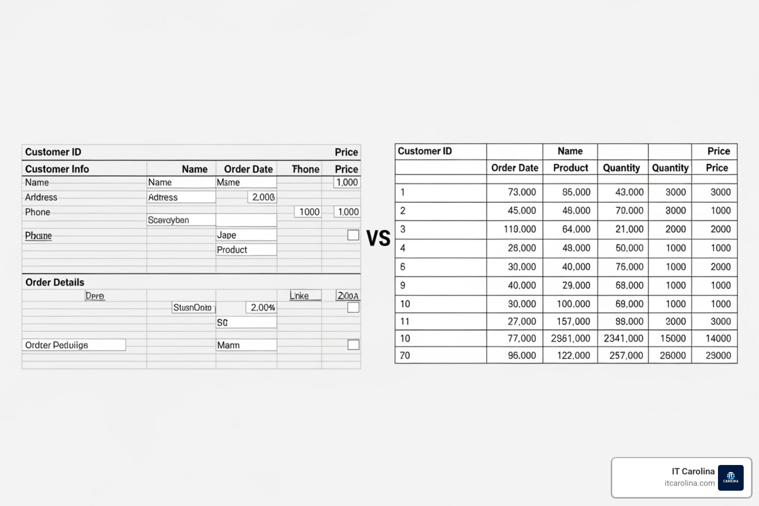
Perhaps the most damaging foundational error is organizing data in a way that makes sense visually but not to Excel. For example, creating separate columns for “Sales Q1,” “Sales Q2,” etc., instead of a single “Sales” column and a “Quarter” column.
This non-tabular layout makes it impossible to use powerful tools like PivotTables, which require “flat” data where each row is a single record and each column is a specific variable. Charting becomes a manual nightmare, and every new question requires reorganizing your data.
The solution is to follow a tabular structure:
- One record per row: Each row contains one complete observation (e.g., one sale).
- One piece of information per cell: Don’t combine data points.
- One column per variable: Each column represents a distinct attribute (e.g., “Date,” “Product,” “Sales Amount”).
If your data is already in a non-tabular format, Excel’s Power Query tool can help you “unpivot” it into the correct structure, making it ready for analysis.

Data & Formula Fails: The Top 10 mistakes you always do in excel spreadsheets
Once your layout is sorted, the next wave of trouble comes from how you enter data and build formulas. These issues are consistently among the top 10 mistakes you always do in excel spreadsheets because they quietly corrupt your calculations.
Mistake #4: Inconsistent Data Entry (Dates and Numbers as Text)
One of the trickiest problems is data that looks like a number or date but is secretly stored as text. Excel sees “5000” or “1/15/2023” as a meaningless string, not a value. As a result, functions like SUM() or AVERAGE() ignore these cells, leading to incorrect totals. Sorting by date also fails, as Excel sorts text alphabetically (“10/1/2022” comes before “2/1/2023”).
To fix this, you first need to spot it. Look for a small green triangle in the corner of the cell. You can also use the ISNUMBER() function to check the data type. To convert the data, the Text to Columns feature (under the Data tab) is highly effective. For numbers, a simple trick is to multiply the column by 1 in a helper column (=A1*1).
The best solution is prevention. Use Excel’s Data Validation tool to set rules that only allow specific data types (like dates or whole numbers) to be entered in a column. If you need help cleaning up a messy dataset, our Online PC Support Services team can assist.
Mistake #5: Hardcoding Numbers Directly into Formulas
It’s tempting to type a value like a tax rate directly into a formula (e.g., =B2*0.05). The problem arises when that value changes. You then have to hunt down every formula where you hardcoded 0.05 and update it manually. This is time-consuming and error-prone; miss one, and your calculations are wrong.
The solution is to store constants in dedicated cells. Create an “Assumptions” section and place your tax rate in a cell, say C1. Then, reference that cell in your formula: =B2*$C$1. For even greater clarity, use Named Ranges. By naming cell C1 as TaxRate, your formula becomes =B2*TaxRate, which is instantly understandable.
When the rate changes, you only need to update one cell, and every formula updates automatically. This makes your spreadsheets flexible, accurate, and easy to maintain. For more ways to work smarter, check out our 15 Computer Tips & Tricks to Master Your Windows Laptop.
Mistake #6: Forgetting Absolute References ($) When Copying Formulas
When you build a perfect formula and drag it down a column, do the results suddenly go wrong? This is often due to forgetting absolute references.
By default, Excel uses relative references, meaning cell addresses adjust as you copy a formula. Sometimes this is what you want, but other times you need a reference to stay locked on a specific cell (like the tax rate cell from the previous example).
For instance, if your formula is =B2*C1 (where C1 is the tax rate), dragging it down changes it to =B3*C2, which is incorrect. The reference to C1 should have been “absolute.”
The solution is the dollar sign ($). An absolute reference like $C$1 will not change when copied. A mixed reference like $C1 locks the column, while C$1 locks the row. The F4 key is your best friend here; while editing a formula, click on a cell reference and press F4 to cycle through the reference types. The correct formula for our example would be =B2*$C$1, ensuring accurate calculations down the entire column.
Advanced Pitfalls: Errors in Data Management and Auditing
Beyond layout and formulas, another layer of errors can creep into spreadsheets. These advanced pitfalls involve how we manage and verify our data, and they can have far-reaching consequences.
Mistake #7: Not Using Excel Tables for Your Data
Many users treat their data as a simple range of cells, missing out on one of Excel’s most powerful features. Without using a proper Excel Table, formulas don’t automatically expand to include new data, charts need to be manually updated, and formatting is inconsistent.
The fix is simple: press Ctrl + T while a cell in your data is selected. This converts your range into an intelligent, dynamic Table. The benefits are immediate:
- Dynamic Ranges: Formulas and charts referencing the table automatically update when you add or remove data.
- Auto-Formatting: New rows inherit the table’s formatting.
- Structured References: Formulas use clear column names like
=SUM(Table1[Sales Amount])instead of cryptic cell ranges like=SUM(B2:B100). - Easy Filtering: Filter buttons are added to headers automatically, and you can use Slicers for interactive dashboards.
Once you start using Tables, you’ll wonder how you ever managed without them.

Mistake #8: Ignoring or Forgetting About Hidden Data
Hiding rows or columns to simplify a view is common, but forgetting they exist is dangerous, especially when sharing files. Hidden data isn’t gone, and it can lead to serious security and data integrity issues.
The risks are real. Sensitive information like salaries or client details can be accidentally shared. Barclays Capital famously “bought 179 contracts they didn’t want… due to hidden rows in an Excel report.” Furthermore, copying and pasting from a range with hidden cells often includes the hidden data, leading to confusion and errors.
The solution is vigilance. Before sharing any file, unhide all rows and columns to review what’s there. If data is sensitive or irrelevant, delete it—don’t just hide it. If you need to copy only the visible cells from a filtered list, select the range, press Ctrl + G, click “Special,” choose “Visible cells only,” and then copy. This practice is a key part of good Cybersecurity Tips for Small Businesses: Protect Your Data.
Mistake #9: Manually Summarizing Data Instead of Using Raw Data
When asked for a monthly summary from daily sales data, many people create a new sheet and manually sum up the figures. This approach destroys valuable detail and locks you into a single view. If someone then asks for a weekly breakdown or a summary by product, you have to start over.
Manual summarization is also error-prone, as it’s easy to miss a row or define a formula range incorrectly. The research from the ICAEW’s Twenty principles for good spreadsheet practice emphasizes keeping raw data pristine.
The better approach is to preserve your raw data in a clean, tabular format (ideally an Excel Table) and let Excel do the summarizing. PivotTables are your best friend here. They allow you to create dynamic summaries that can be sliced, diced, and reconfigured in seconds without altering your original data. Alternatively, functions like SUMIFS() and COUNTIFS() can pull summary figures directly from your raw data sheet.
Mistake #10: Failing to Manually Audit Formulas and Results
Just because a spreadsheet produces numbers doesn’t mean they are correct. Human error is inevitable, and unaudited formulas can lead to catastrophic results, like JP Morgan’s $6 billion trading loss or Public Health England’s loss of 16,000 COVID-19 test records.
Some errors don’t even show up as #VALUE!; they just produce a plausible but incorrect number that can inform poor business decisions.
You must develop a habit of auditing your work.
- Spot-check results: Manually verify a few calculations with a calculator.
- Review with fresh eyes: Step away and come back later. You’re more likely to catch mistakes.
- Use Formula Auditing tools: On the Formulas tab, use Trace Precedents (to see what cells a formula uses), Trace Dependents (to see where a cell’s value is used), and Show Formulas to review all logic at once.
Auditing takes a little extra time, but it’s critical for ensuring accuracy. If you need an expert to review complex spreadsheets, Get professional Charlotte tech support from IT Carolina.
Frequently Asked Questions about Common Excel Mistakes
How can I quickly fix dates that are formatted as text?
The fastest method is the Text to Columns feature. Select the column with the text-formatted dates, go to the Data tab, and click “Text to Columns.” In the wizard’s third step, select “Date” and choose the format that matches your data (e.g., MDY for Month/Day/Year). Click “Finish,” and Excel will convert the text to proper dates.
Alternatively, you can use a formula in a helper column. Functions like =DATEVALUE(A1) or even a simple mathematical operation like =A1+0 can force the conversion. After using a formula, copy the results and use “Paste Values” to finalize them. For more help with Excel issues, our Online PC Support Services are available.
What is the biggest risk of the top 10 mistakes you always do in excel spreadsheets?
The biggest risk is significant financial loss and compromised data integrity. These aren’t minor issues; they have led to real-world disasters. For example, a copy-paste error in an Excel model cost JP Morgan $6 billion, and TransAlta Corp lost $24 million due to misaligned rows in a spreadsheet.
Other incidents, like Public Health England losing nearly 16,000 COVID-19 test results because of Excel’s row limit, show that the consequences can extend beyond financial loss to operational and public safety failures. These cautionary tales highlight why avoiding the Top 10 mistakes you always do in excel spreadsheets is so critical.
What is a better alternative to merging cells for a title?
The best alternative is “Center Across Selection.” It provides the same centered look as merging cells but doesn’t break Excel’s grid structure, so sorting, filtering, and copying continue to work perfectly.
To use it, select the cells you want the title to span (e.g., A1 through D1). Press Ctrl + 1 to open the “Format Cells” dialog. On the “Alignment” tab, choose “Center Across Selection” from the “Horizontal” alignment dropdown and click “OK.” Your title will be centered without causing any of the frustrating problems associated with merged cells.
Conclusion: From Excel Novice to Pro
We’ve explored the Top 10 mistakes you always do in excel spreadsheets, from simple formatting errors like merging cells to critical oversights like skipping formula audits. Each mistake carries real consequences, capable of derailing analysis, wasting time, and even causing financial disasters measured in the millions.
The examples of JP Morgan’s $6 billion loss and Public Health England’s misplaced test results are stark reminders that our spreadsheets matter. The data we manage directly impacts the decisions we make.
The encouraging news is that these errors are avoidable. You don’t need to be an Excel wizard; you just need to build better habits. Use “Center Across Selection,” convert data to Excel Tables (Ctrl + T), preserve your raw data, use absolute references ($), and always audit your formulas. These small practices transform your spreadsheets from brittle and error-prone to robust and reliable.
By adopting these habits, you spend less time fighting mysterious errors and more time gaining valuable insights. That is the true path from Excel novice to pro.
Of course, technology can still be challenging. When you’re stuck on a complex formula or dealing with other computer issues, you don’t have to go it alone. IT Carolina offers friendly, jargon-free support to help you steer the digital world. Get professional Charlotte tech support whenever you need a hand—we’re here to help you succeed.